Adjunctive echinocandin plus TMP-SMX versus TMP-SMX monotherapy for Pneumocystis pneumonia in HIV-negative adults: an interim Bayesian meta-analysis

library(tidyverse)

── Attaching core tidyverse packages ──────────────────────── tidyverse 2.0.0 ──
✔ dplyr     1.2.1     ✔ readr     2.2.0
✔ forcats   1.0.1     ✔ stringr   1.6.0
✔ ggplot2   4.0.3     ✔ tibble    3.3.1
✔ lubridate 1.9.5     ✔ tidyr     1.3.2
✔ purrr     1.2.2     
── Conflicts ────────────────────────────────────────── tidyverse_conflicts() ──
✖ dplyr::filter() masks stats::filter()
✖ dplyr::lag()    masks stats::lag()
ℹ Use the conflicted package (<http://conflicted.r-lib.org/>) to force all conflicts to become errors

library(metafor)

Loading required package: Matrix

Attaching package: 'Matrix'

The following objects are masked from 'package:tidyr':

    expand, pack, unpack

Loading required package: metadat
Loading required package: numDeriv

Loading the 'metafor' package (version 5.0-1). For an
introduction to the package please type: help(metafor)

library(bayesmeta)

Loading required package: forestplot
Loading required package: grid
Loading required package: checkmate
Loading required package: abind
Loading required package: mvtnorm

Attaching package: 'bayesmeta'

The following object is masked from 'package:stats':

    convolve

source("analysis/jama_style.R")

# Verified analysis dataset (source-checked counts). One row per study:
# combination (echinocandin) arm events/N and reference (monotherapy) arm events/N.
ma <- read_csv("analysis/pcp_primary_meta_dataset.csv", show_col_types = FALSE) |>
  select(study, tier, timing, timepoint, e_comb, n_comb, e_ref, n_ref)

# Recompute per-study log odds ratios from the raw counts (self-contained).
ma <- escalc(measure = "OR",
             ai = e_comb, n1i = n_comb,   # combination (echinocandin) arm
             ci = e_ref,  n2i = n_ref,    # reference (monotherapy) arm
             data = ma, slab = study) |>
  mutate(sei = sqrt(vi), OR = exp(yi))

# Bayesian random-effects (normal-normal) meta-analysis with weakly informative
# priors: mu ~ N(0, 1.5) on the log-OR; tau ~ half-normal(0.5).
fit_bm <- function(d) {
  bayesmeta(y = d$yi, sigma = d$sei, labels = d$study,
            mu.prior  = c(mean = 0, sd = 1.5),
            tau.prior = function(t) dhalfnormal(t, scale = 0.5))
}
or_ci <- function(bm) c(exp(bm$summary["median", "mu"]),
                        exp(bm$summary["95% lower", "mu"]),
                        exp(bm$summary["95% upper", "mu"]))
fmt   <- function(bm) { v <- or_ci(bm); sprintf("%.2f (95%% CrI %.2f\u2013%.2f)", v[1], v[2], v[3]) }
plt1  <- function(bm) bm$pposterior(mu = 0)   # P(OR < 1 | data)

bm_primary <- fit_bm(filter(ma, tier == "primary"))      # k = 3
bm_sens    <- fit_bm(ma)                                  # k = 6
bm_initial <- fit_bm(filter(ma, timing == "initial"))    # Jin2019, Qi2023, Li2024a
bm_mixed   <- fit_bm(filter(ma, timing == "mixed"))       # Qi2025, Xu2025, Lu2017

Background and objective

This review addresses the PROSPERO-registered question of the comparative effectiveness of combination and adjunctive regimens versus standard monotherapy for Pneumocystis jirovecii pneumonia (PCP/PJP) in HIV-negative / immunocompromised adults. The most coherent contrast supported by the currently available data is adjunctive echinocandin/caspofungin plus trimethoprim-sulfamethoxazole (TMP-SMX) versus TMP-SMX monotherapy, with all-cause mortality (30-day and/or in-hospital) as the primary outcome, expressed as an odds ratio (OR) with 95% credible intervals (CrI).

Methods

Data source and verification

Study-level data were extracted from a structured extraction database (machine first-pass) and then verified against the source full texts before analysis. Verification changed the analytic set in three material ways:

• Tian2020 was excluded: it is an HIV-positive cohort (published in HIV Medicine), which violates the HIV-negative inclusion criterion. The machine draft had misclassified it.
• Qi2025 and Yanmeng2026 are the same PUMCH cohort (byte-identical source); one copy was retained. The full-cohort comparison (Table 4: 18/35 caspofungin vs 31/79 monotherapy) was used, not the mechanically-ventilated subgroup.
• Li2024a was retained but flagged confounded: its combination arm bundles caspofungin with a corticosteroid and a lower TMP dose, so it cannot isolate an echinocandin effect. It sits in the sensitivity tier only.

The primary analysis comprises the studies reporting in-hospital or ~30-day mortality (Qi2025, Xu2025, Lu2017); the sensitivity analysis adds studies reporting longer-timepoint mortality (Jin2019, Qi2023, Li2024a).

Statistical model

We fitted a Bayesian random-effects (normal-normal) meta-analysis on the per-study log odds ratios, with weakly informative priors: a normal N(0, 1.5) prior on the pooled log-OR and a half-normal(0.5) prior on the between-study standard deviation \[\tau\]. Models were fitted with the bayesmeta package, which integrates the posterior semi-analytically (no MCMC). This choice was necessary because the Stan toolchain is unavailable on the analysis machine; the trade-off is that we use a two-stage normal approximation rather than an exact binomial-likelihood hierarchical model, which is less ideal for the sparse cells in the smallest studies.

Results

Included studies

ma |>
  transmute(Study = study, Tier = tier, Timing = timing, Timepoint = timepoint,
            `Combination (events/N)` = paste0(e_comb, "/", n_comb),
            `Monotherapy (events/N)` = paste0(e_ref, "/", n_ref),
            OR = round(OR, 2)) |>
  knitr::kable()

Study	Tier	Timing	Timepoint	Combination (events/N)	Monotherapy (events/N)	OR
Qi2025	primary	mixed	in-hospital	18/35	31/79	1.64
Xu2025	primary	mixed	28-day	33/89	19/31	0.37
Lu2017	primary	mixed	episode/in-hosp	1/5	2/6	0.50
Jin2019	sensitivity	initial	3-month	8/35	33/91	0.52
Qi2023	sensitivity	initial	90-day	17/43	10/21	0.72
Li2024a	sensitivity	initial	episode (unspec)	5/20	3/18	1.67

Primary and sensitivity estimates

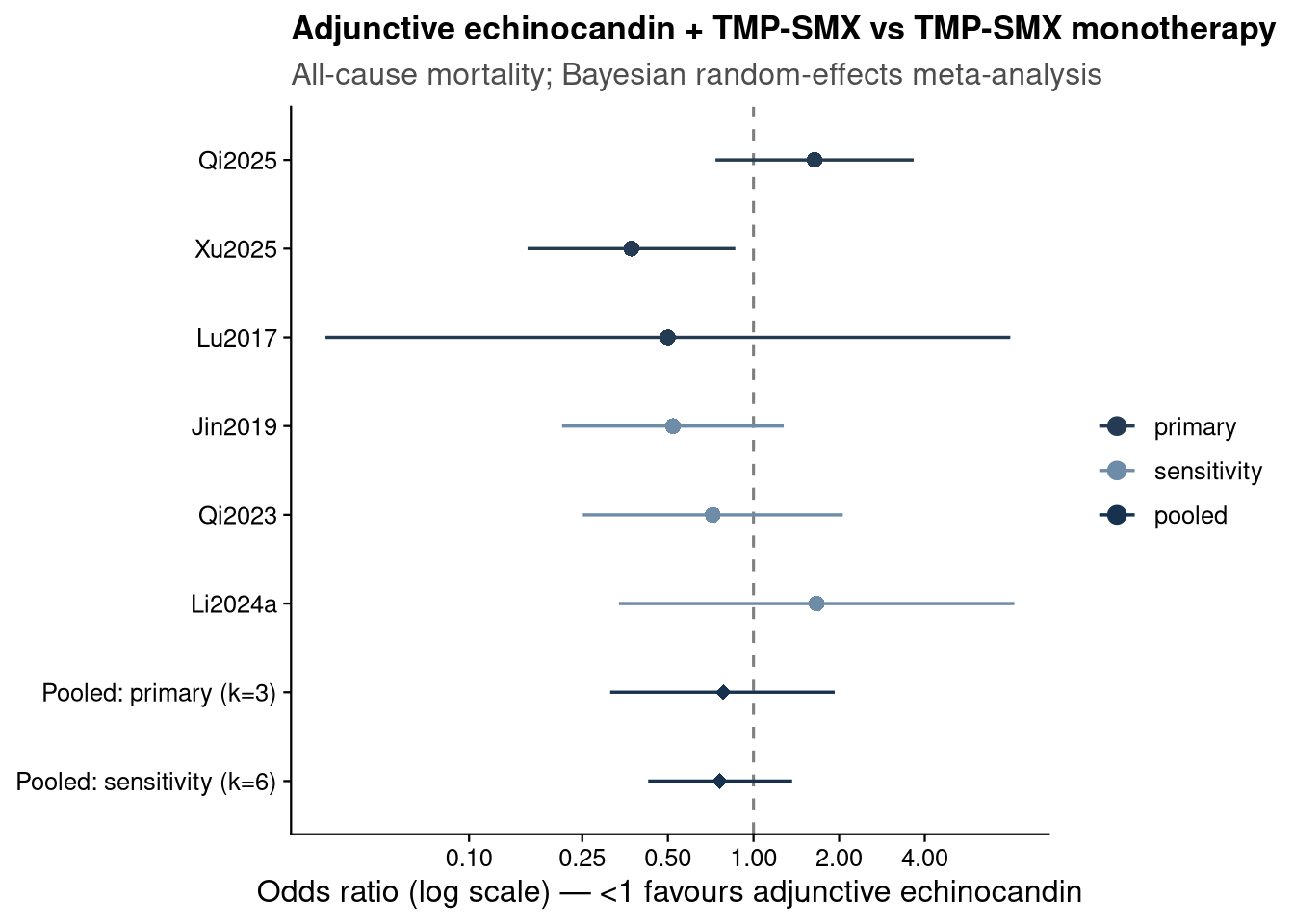
The primary analysis (k = 3) gives a pooled OR of 0.78 (95% CrI 0.31–1.93), and the sensitivity analysis (k = 6) gives 0.76 (95% CrI 0.43–1.37) (posterior probability that OR < 1 = 0.84). Both estimates point toward a possible mortality reduction with adjunctive echinocandin, but both credible intervals include OR = 1, so the evidence is suggestive rather than conclusive.

study_fp <- ma |>
  transmute(label = study, tier,
            OR = exp(yi), lo = exp(yi - 1.96 * sei), hi = exp(yi + 1.96 * sei))
pooled_fp <- tibble(
  label = c("Pooled: primary (k=3)", "Pooled: sensitivity (k=6)"),
  tier  = "pooled",
  OR = c(or_ci(bm_primary)[1], or_ci(bm_sens)[1]),
  lo = c(or_ci(bm_primary)[2], or_ci(bm_sens)[2]),
  hi = c(or_ci(bm_primary)[3], or_ci(bm_sens)[3]))

bind_rows(study_fp, pooled_fp) |>
  mutate(label = factor(label, levels = rev(c(
           "Qi2025", "Xu2025", "Lu2017", "Jin2019", "Qi2023", "Li2024a",
           "Pooled: primary (k=3)", "Pooled: sensitivity (k=6)"))),
         tier = factor(tier, levels = c("primary", "sensitivity", "pooled"))) |>
  ggplot(aes(OR, label, color = tier)) +
  geom_vline(xintercept = 1, linetype = "dashed", color = "grey50") +
  geom_pointrange(aes(xmin = lo, xmax = hi, shape = tier == "pooled"), linewidth = 0.6) +
  scale_x_log10(breaks = c(0.1, 0.25, 0.5, 1, 2, 4)) +
  scale_color_manual(values = jama_tier) +
  scale_shape_manual(values = c(16, 18), guide = "none") +
  labs(x = "Odds ratio (log scale) \u2014 <1 favours adjunctive echinocandin", y = NULL,
       title = "Adjunctive echinocandin + TMP-SMX vs TMP-SMX monotherapy",
       subtitle = "All-cause mortality; Bayesian random-effects meta-analysis") +
  theme_jama()

Timing subgroups

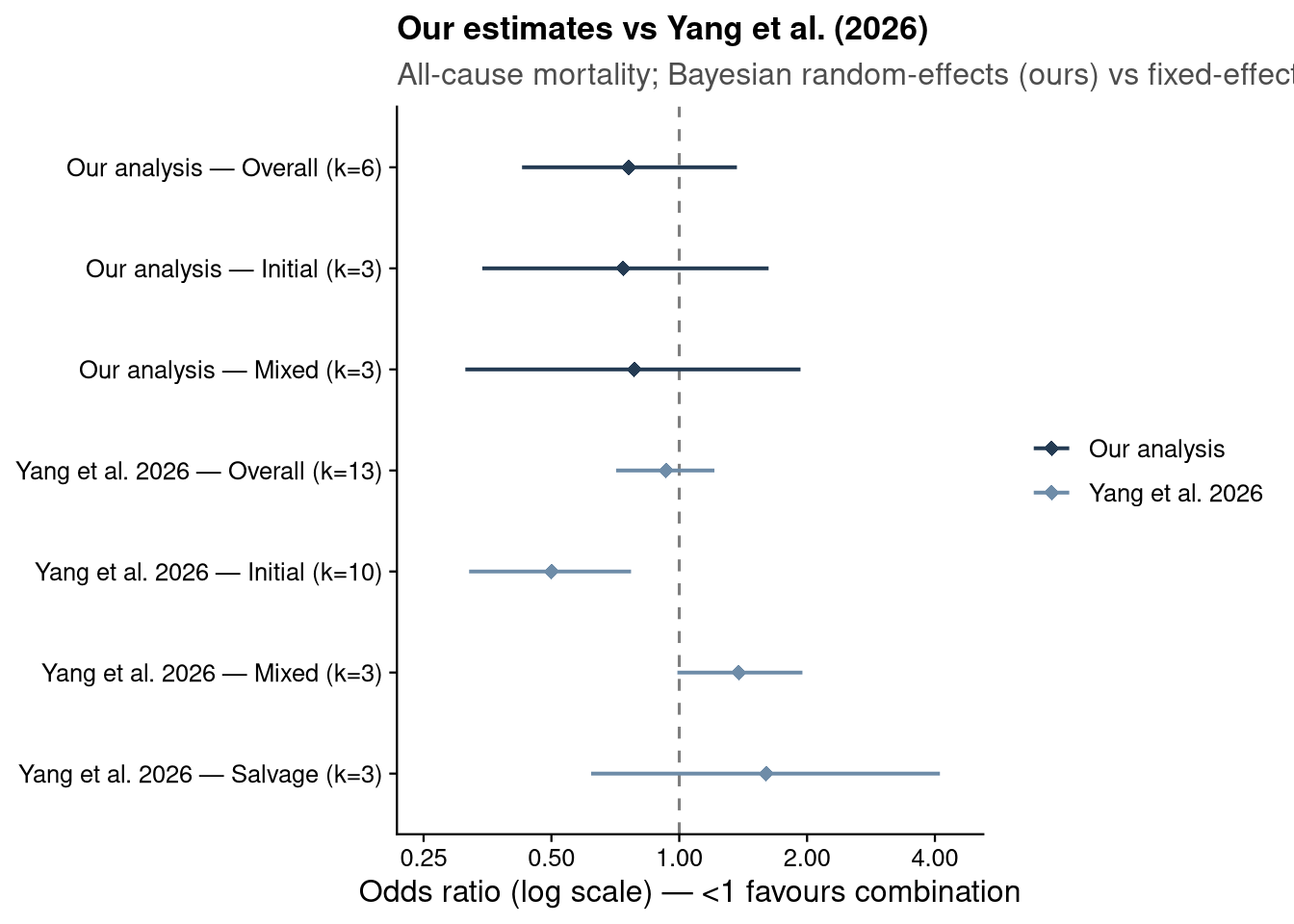
Following Yang et al. (2026), studies were classified by treatment timing (initial vs mixed; no pure salvage-vs-monotherapy study is available in our set). The initial-strategy subgroup (k = 3) gives 0.74 (95% CrI 0.34–1.62) and the mixed-strategy subgroup (k = 3) gives 0.78 (95% CrI 0.31–1.93). Both remain inconclusive. Our strict initial subgroup is less protective than Yang’s because we classified Xu2025 (a strong-benefit study) as mixed, consistent with its source (caspofungin timing not restricted to first-line; “selection bias in caspofungin use” acknowledged).

Comparison with Yang et al. (2026)

Yang et al. asked the same question with a broader search (including Chinese databases). We share 9 of their 16 studies. Their overall estimate is null (OR 0.93) but their initial-strategy subgroup is clearly protective (OR 0.50); the figure below places our estimates alongside theirs. The two analyses are consistent once treatment timing is matched.

comp <- tibble(
  source   = c(rep("Our analysis", 3), rep("Yang et al. 2026", 4)),
  subgroup = c("Overall", "Initial", "Mixed", "Overall", "Initial", "Mixed", "Salvage"),
  k        = c(6, 3, 3, 13, 10, 3, 3),
  OR = c(or_ci(bm_sens)[1], or_ci(bm_initial)[1], or_ci(bm_mixed)[1], 0.93, 0.50, 1.38, 1.60),
  lo = c(or_ci(bm_sens)[2], or_ci(bm_initial)[2], or_ci(bm_mixed)[2], 0.71, 0.32, 0.99, 0.62),
  hi = c(or_ci(bm_sens)[3], or_ci(bm_initial)[3], or_ci(bm_mixed)[3], 1.21, 0.77, 1.95, 4.11)) |>
  mutate(row = paste0(source, " \u2014 ", subgroup, " (k=", k, ")"))
comp$row <- factor(comp$row, levels = rev(comp$row))

ggplot(comp, aes(OR, row, color = source)) +
  geom_vline(xintercept = 1, linetype = "dashed", color = "grey50") +
  geom_pointrange(aes(xmin = lo, xmax = hi), shape = 18, linewidth = 0.7) +
  scale_x_log10(breaks = c(0.25, 0.5, 1, 2, 4), limits = c(0.25, 4.5)) +
  scale_color_manual(values = c("Our analysis" = jama_blue_grey[["dark"]],
                                "Yang et al. 2026" = jama_blue_grey[["medium"]])) +
  labs(x = "Odds ratio (log scale) \u2014 <1 favours combination", y = NULL,
       title = "Our estimates vs Yang et al. (2026)",
       subtitle = "All-cause mortality; Bayesian random-effects (ours) vs fixed-effect M-H (Yang)") +
  theme_jama()

Note that Yang et al.’s extraction contains errors we identified during verification, so it is a useful comparator rather than a ground truth: their Qi2025 numbers come from the ventilated subgroup, and their “Wang 2019” entry treats a single-arm case series (9 patients, 0 deaths) as a two-arm comparison.

Robustness: leave-one-out

loo <- map_dfr(ma$study, function(s) {
  bm <- fit_bm(filter(ma, study != s))
  tibble(removed = paste0("\u2212 ", s),
         OR = exp(bm$summary["median", "mu"]),
         lo = exp(bm$summary["95% lower", "mu"]),
         hi = exp(bm$summary["95% upper", "mu"]))
})
loo <- bind_rows(
  tibble(removed = "Full model (k=6)",
         OR = or_ci(bm_sens)[1], lo = or_ci(bm_sens)[2], hi = or_ci(bm_sens)[3]),
  loo)
loo |> mutate(across(where(is.numeric), ~round(.x, 2))) |> knitr::kable()

removed	OR	lo	hi
Full model (k=6)	0.76	0.43	1.37
− Qi2025	0.59	0.32	1.09
− Xu2025	0.94	0.50	1.76
− Lu2017	0.77	0.42	1.43
− Jin2019	0.84	0.43	1.66
− Qi2023	0.77	0.39	1.53
− Li2024a	0.70	0.38	1.31

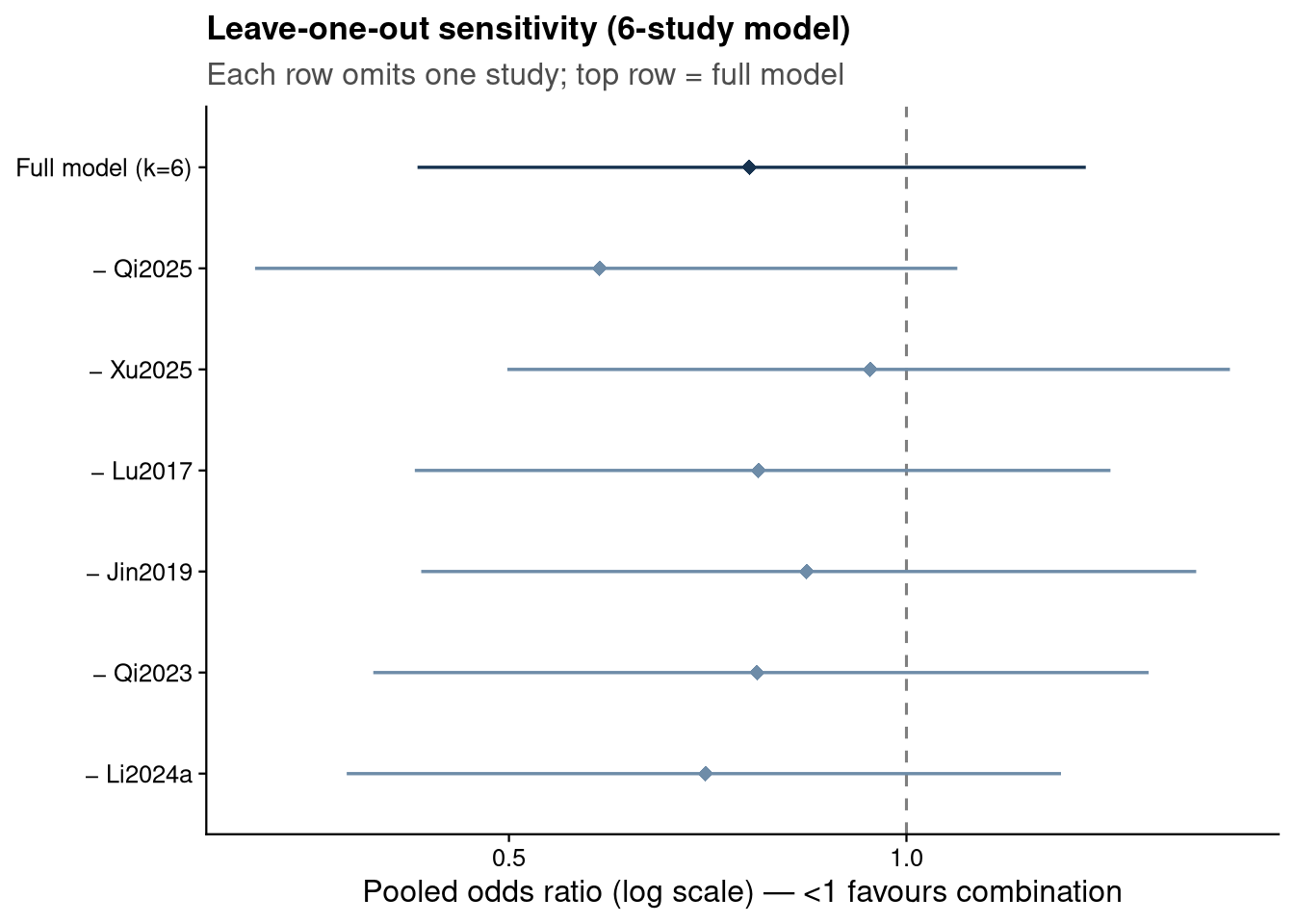
The pooled OR ranges from about 0.59 (omitting Qi2025) to 0.94 (omitting Xu2025). Every leave-one-out estimate still crosses OR = 1, so no single study changes the qualitative conclusion, but Xu2025 is the single most influential study, accounting for most of the apparent benefit.

loo |>
  mutate(kind = ifelse(removed == "Full model (k=6)", "full", "loo"),
         removed = factor(removed, levels = rev(removed))) |>
  ggplot(aes(OR, removed, color = kind)) +
  geom_vline(xintercept = 1, linetype = "dashed", color = "grey50") +
  geom_pointrange(aes(xmin = lo, xmax = hi), shape = 18, linewidth = 0.6) +
  scale_x_log10(breaks = c(0.25, 0.5, 1, 2)) +
  scale_color_manual(values = c(full = jama_blue_grey[["accent"]],
                                loo  = jama_blue_grey[["medium"]]), guide = "none") +
  labs(x = "Pooled odds ratio (log scale) \u2014 <1 favours combination", y = NULL,
       title = "Leave-one-out sensitivity (6-study model)",
       subtitle = "Each row omits one study; top row = full model") +
  theme_jama()

Robustness: prior sensitivity

fit_prior <- function(mu_sd, tau_scale, fam) {
  tp <- switch(fam,
    HN = function(t) dhalfnormal(t, scale = tau_scale),
    HC = function(t) dhalfcauchy(t, scale = tau_scale),
    U  = function(t) dunif(t, 0, tau_scale))
  bayesmeta(y = ma$yi, sigma = ma$sei, labels = ma$study,
            mu.prior = c(mean = 0, sd = mu_sd), tau.prior = tp)
}
grid <- tribble(
  ~prior,                            ~mu_sd, ~tau_scale, ~fam,
  "Base: mu~N(0,1.5), tau~HN(0.5)",     1.5,  0.50, "HN",
  "Tighter tau ~ HN(0.25)",             1.5,  0.25, "HN",
  "Wider tau ~ HN(1.0)",                1.5,  1.00, "HN",
  "tau ~ half-Cauchy(0.5)",             1.5,  0.50, "HC",
  "tau ~ Uniform(0,2)",                 1.5,  2.00, "U",
  "Wider mu ~ N(0,10)",                  10,  0.50, "HN",
  "Tighter mu ~ N(0,1)",                1.0,  0.50, "HN")

pmap_dfr(list(grid$prior, grid$mu_sd, grid$tau_scale, grid$fam),
  function(p, m, ts, f) {
    bm <- fit_prior(m, ts, f)
    tibble(Prior = p,
           OR = exp(bm$summary["median", "mu"]),
           lo = exp(bm$summary["95% lower", "mu"]),
           hi = exp(bm$summary["95% upper", "mu"]),
           tau = bm$summary["median", "tau"])
  }) |>
  mutate(across(where(is.numeric), ~round(.x, 2))) |>
  knitr::kable()

Prior	OR	lo	hi	tau
Base: mu~N(0,1.5), tau~HN(0.5)	0.76	0.43	1.37	0.37
Tighter tau ~ HN(0.25)	0.76	0.47	1.23	0.22
Wider tau ~ HN(1.0)	0.76	0.39	1.53	0.49
tau ~ half-Cauchy(0.5)	0.76	0.41	1.41	0.38
tau ~ Uniform(0,2)	0.77	0.36	1.66	0.57
Wider mu ~ N(0,10)	0.75	0.42	1.37	0.37
Tighter mu ~ N(0,1)	0.77	0.44	1.36	0.37

The pooled OR is essentially invariant to the prior specification (0.75–0.77 across all choices). Only the credible-interval width responds to the heterogeneity prior, as expected: a tighter \[\tau\] prior narrows the interval and a uniform prior widens it. The pooled location is therefore robust; the residual uncertainty is driven by the small number of studies and genuine between-study heterogeneity rather than by prior choice.

Limitations

• Missing Chinese-language studies. Yang et al.’s broader search (CNKI/Wanfang) captured several Chinese-language papers and two master’s theses (Li2015, Liu2015, Wang2021, Wu2023, Xiang2015) plus Yu2017 (a discontinued journal) that we could not retrieve. Their absence limits power and could introduce language/selection bias relative to a complete corpus. (Wang ZG 2019, also missing from our set, was obtained and found ineligible — a single-arm case series with no comparator.)
• Extraction provenance. The source database is a machine first-pass. Counts for the included studies were verified against source text, but full dual human verification is still pending.
• Observational data and confounding. All included studies are observational; treatment was clinician-assigned, so confounding by indication is likely. This is most acute for Xu2025 — the most influential study — whose monotherapy arm was sicker (more solid tumour and aspergillosis co-infection).
• Small k and heterogeneous timepoints. With three to six studies and mortality measured over differing windows (in-hospital, 28-day, 90-day, 3-month), pooled estimates are imprecise and heterogeneity is difficult to characterise.
• Confounded and non-estimable comparisons. Li2024a bundles caspofungin with corticosteroid and a lower TMP dose. Near-universal corticosteroid use across studies precludes a corticosteroid presence/absence subgroup, and only one small study omitted β-D-glucan, so those planned sub-analyses were not estimable.
• Model approximation. Because Stan was unavailable, we used a two-stage normal-normal model rather than an exact binomial hierarchical model, which is less ideal for the sparse cells in the smallest studies (e.g., Lu2017).

Conclusion

In source-verified, HIV-negative PCP cohorts, adjunctive echinocandin plus TMP-SMX shows a possible but inconclusive mortality benefit versus TMP-SMX monotherapy (sensitivity OR 0.76 (95% CrI 0.43–1.37)). The direction is consistent with Yang et al.’s initial-therapy signal once timing is matched, but the credible intervals include no effect, the result is sensitive to a single influential study (Xu2025), and the evidence base is small, observational, and incomplete. Higher-quality data — ideally the missing Chinese-language studies and, ultimately, randomized evidence — are needed before drawing a firm conclusion.