Model fit and MCMC convergence

source("analysis/meta_helpers.R")
library(coda)
ma <- load_ma()

Note

Preliminary, machine-assisted output pending human review.

The model

The headline Bayesian estimates (Bayesian page) are computed semi-analytically by bayesmeta and therefore do not involve MCMC. To provide genuine sampler diagnostics — and an independent check of that computation — we refit the identical model by MCMC using a self-contained random-walk Metropolis sampler written in base R (no JAGS or Stan dependency).

For studies \[i = 1, \dots, k\] with observed log odds ratio \[y_i\] and standard error \[s_i\]:

\[y_i \sim \mathrm{Normal}(\theta_i,\ s_i^2), \qquad \theta_i \sim \mathrm{Normal}(\mu,\ \tau^2)\]

with weakly informative priors \[\mu \sim \mathrm{Normal}(0, 1.5^2)\] and \[\tau \sim \mathrm{half\text{-}Normal}(0.5)\]. The pooled odds ratio is \[\mathrm{OR} = e^{\mu}\]. The study effects \[\theta_i\] are integrated out analytically, so the sampler targets the marginal posterior of \[(\mu, \tau)\]. We ran 4 chains — 3000 burn-in iterations (during which the proposal covariance is adapted) followed by 10,000 retained iterations per chain.

s <- fit_mcmc(ma)

Convergence diagnostics

rhat <- gelman.diag(s[, c("mu", "tau")], multivariate = FALSE)$psrf
ess  <- effectiveSize(s[, c("mu", "tau", "OR")])

tibble(Parameter = c("mu (log-OR)", "tau"),
       `R-hat` = round(rhat[, 1], 3),
       `R-hat upper CI` = round(rhat[, 2], 3),
       `Effective sample size` = round(ess[c("mu", "tau")])) |>
  knitr::kable()

Parameter	R-hat	R-hat upper CI	Effective sample size
mu (log-OR)	1.001	1.003	3751
tau	1.001	1.002	4540

All potential scale reduction factors (R̂) are at or very close to 1.00 and effective sample sizes are in the thousands, indicating the chains have converged and mixed well.

Trace and density

draws <- purrr::imap_dfr(s, function(chain, i)
  as_tibble(as.matrix(chain)[, c("mu", "tau")]) |>
    mutate(chain = factor(i), iter = row_number()))
draws_long <- pivot_longer(draws, c(mu, tau), names_to = "parameter", values_to = "value")

ggplot(draws_long, aes(iter, value, color = chain)) +
  geom_line(alpha = 0.6, linewidth = 0.25) +
  facet_wrap(~ parameter, ncol = 1, scales = "free_y") +
  scale_color_manual(values = jama_chains) +
  labs(x = "Iteration", y = NULL, title = "Trace plots (4 chains)") +
  theme_jama()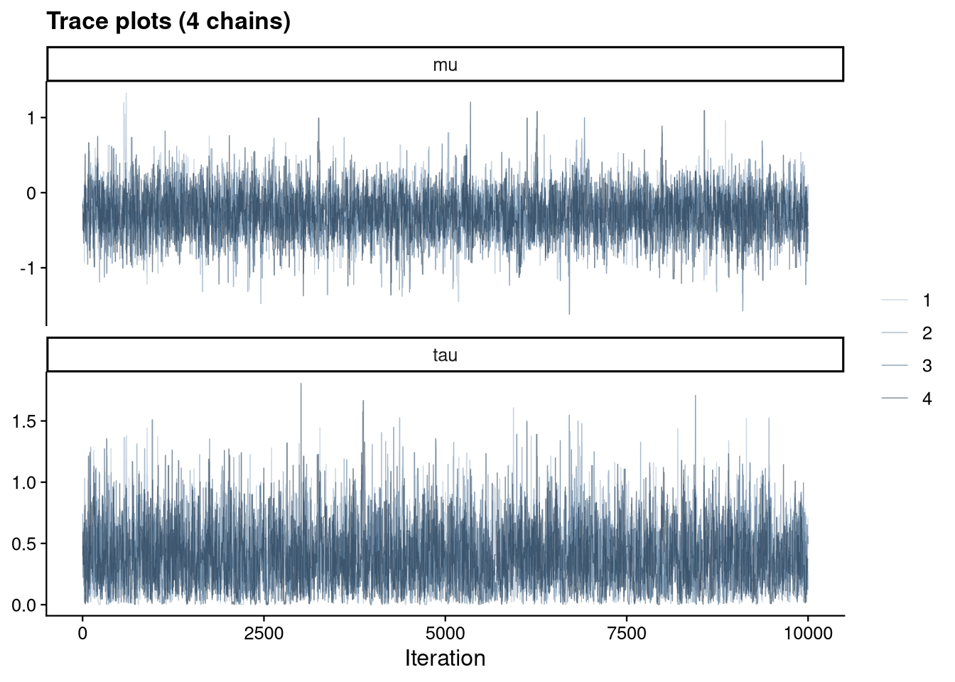

ggplot(draws_long, aes(value, color = chain)) +
  geom_density() +
  facet_wrap(~ parameter, ncol = 2, scales = "free") +
  scale_color_manual(values = jama_chains) +
  labs(x = NULL, y = "Density", title = "Posterior density by chain") +
  theme_jama()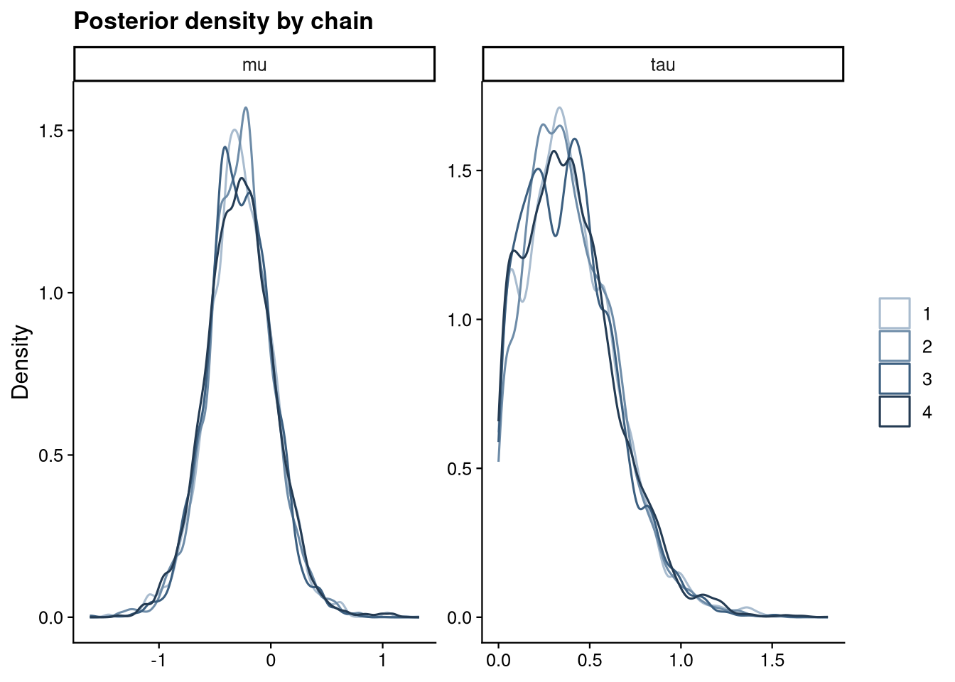

The chains are indistinguishable, with no drift or stickiness in the traces and overlapping per-chain densities.

Cross-check: MCMC vs bayesmeta

bm_sens  <- fit_bm(ma)
mcmc_or  <- exp(summary(s)$quantiles["mu", c("2.5%", "50%", "97.5%")])
tibble(
  Engine = c("Random-walk Metropolis (MCMC)", "bayesmeta (semi-analytic)"),
  `OR median` = c(mcmc_or[2], or_ci(bm_sens)[1]),
  `CrI lower` = c(mcmc_or[1], or_ci(bm_sens)[2]),
  `CrI upper` = c(mcmc_or[3], or_ci(bm_sens)[3])
) |>
  mutate(across(where(is.numeric), ~round(.x, 3))) |>
  knitr::kable()

Engine	OR median	CrI lower	CrI upper
Random-walk Metropolis (MCMC)	0.758	0.424	1.370
bayesmeta (semi-analytic)	0.760	0.426	1.367

The two independent implementations agree to within Monte Carlo error, confirming the semi-analytic posterior used elsewhere on this site.