Frequentist meta-analysis

source("analysis/meta_helpers.R")
ma <- load_ma()

For comparability with the wider literature (including Yang et al. 2026, who used a fixed-effect Mantel-Haenszel model), we fit a frequentist synthesis alongside the Bayesian analysis. The random-effects model (REML) is the primary frequentist estimate; the Mantel-Haenszel fixed-effect model is shown for comparison.

re <- rma(yi, vi, data = ma, method = "REML")            # random-effects (REML)
mh <- rma.mh(ai = e_comb, n1i = n_comb, ci = e_ref, n2i = n_ref,
             data = ma, measure = "OR")                   # Mantel-Haenszel fixed-effect
re

Random-Effects Model (k = 6; tau^2 estimator: REML)

tau^2 (estimated amount of total heterogeneity): 0.2150 (SE = 0.3269)
tau (square root of estimated tau^2 value):      0.4637
I^2 (total heterogeneity / total variability):   42.10%
H^2 (total variability / sampling variability):  1.73

Test for Heterogeneity:
Q(df = 5) = 7.9981, p-val = 0.1563

Model Results:

estimate      se     zval    pval    ci.lb   ci.ub    
 -0.2814  0.3008  -0.9354  0.3496  -0.8710  0.3082    

---
Signif. codes:  0 '***' 0.001 '**' 0.01 '*' 0.05 '.' 0.1 ' ' 1

Pooled estimates

tibble(
  Model = c("Random-effects (REML)", "Mantel-Haenszel (fixed)"),
  OR = c(exp(re$b[1]), exp(mh$b[1])),
  `95% CI lower` = c(exp(re$ci.lb), exp(mh$ci.lb)),
  `95% CI upper` = c(exp(re$ci.ub), exp(mh$ci.ub))
) |>
  mutate(across(where(is.numeric), ~round(.x, 2))) |>
  knitr::kable()

Model	OR	95% CI lower	95% CI upper
Random-effects (REML)	0.75	0.42	1.36
Mantel-Haenszel (fixed)	0.75	0.50	1.13

The random-effects pooled odds ratio is 0.75 (95% CI 0.42-1.36). Between-study heterogeneity is moderate (I² = 42%, τ² = 0.21; Cochran’s Q = 8.0, p = 0.16). The interval crosses OR = 1, so the effect is not statistically significant.

Forest plot

est <- ma |>
  transmute(label = study, kind = "study",
            OR = exp(yi), lo = exp(yi - 1.96 * sei), hi = exp(yi + 1.96 * sei))
pool <- tibble(
  label = c("Random-effects (REML)", "Mantel-Haenszel (fixed)"), kind = "pooled",
  OR = c(exp(re$b[1]), exp(mh$b[1])),
  lo = c(exp(re$ci.lb), exp(mh$ci.lb)),
  hi = c(exp(re$ci.ub), exp(mh$ci.ub)))

bind_rows(est, pool) |>
  mutate(label = factor(label, levels = rev(c(ma$study,
           "Random-effects (REML)", "Mantel-Haenszel (fixed)")))) |>
  ggplot(aes(OR, label, color = kind)) +
  geom_vline(xintercept = 1, linetype = "dashed", color = "grey50") +
  geom_pointrange(aes(xmin = lo, xmax = hi, shape = kind == "pooled"), linewidth = 0.6) +
  scale_x_log10(breaks = c(0.1, 0.25, 0.5, 1, 2, 4)) +
  scale_color_manual(values = c(study = jama_blue_grey[["medium"]],
                                pooled = jama_blue_grey[["accent"]]), guide = "none") +
  scale_shape_manual(values = c(16, 18), guide = "none") +
  labs(x = "Odds ratio (log scale) \u2014 <1 favours combination", y = NULL,
       title = "Frequentist forest plot",
       subtitle = "Per-study estimates with random-effects and fixed-effect pooled odds ratios") +
  theme_jama()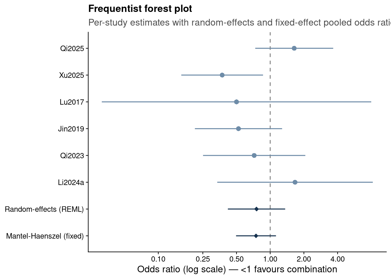

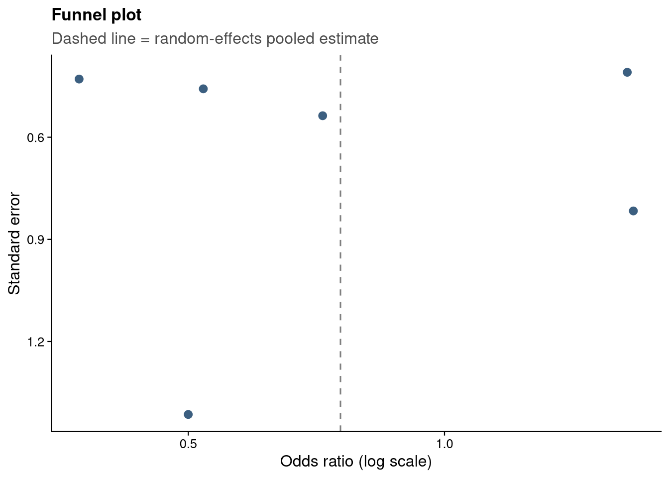
Funnel plot

With only six studies, formal small-study-effect tests (e.g., Egger’s test) are underpowered and not recommended; the funnel plot is shown for completeness only.

ggplot(ma, aes(x = OR, y = sei)) +
  geom_vline(xintercept = exp(re$b[1]), linetype = "dashed", color = "grey50") +
  geom_point(size = 2.4, color = jama_blue_grey[["steel"]]) +
  scale_x_log10(breaks = c(0.25, 0.5, 1, 2, 4)) +
  scale_y_reverse() +
  labs(x = "Odds ratio (log scale)", y = "Standard error",
       title = "Funnel plot",
       subtitle = "Dashed line = random-effects pooled estimate") +
  theme_jama()